Spread Cost Analysis is an essential tool for traders who need to examine the performance of their trading strategies and associated tactics. This data can be used in algo optimisation, pre and post trade analysis and best execution reporting, and can be integrated with portfolio or client level data via the API. Spread Cost Analysis should be used in conjunction with the Order Analysis tool.
Methodology
Spread Cost Analysis measures the difference between the price of a trade and the corresponding mid price at the time of execution and at a series of time offsets. Results are aggregated to summarise the overall efficiency of order placement and are provided at the individual trade level within the tool.
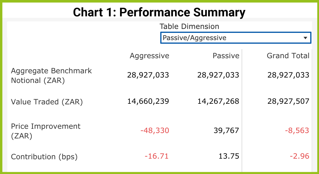
The Performance Summary below shows the trading cost for a simulated trading Firm. Trades are categorised according to whether they originate from orders placed passively on the near touch or aggressively on the far touch. Alternatively they can be viewed as buys and sells.
Price Improvement or Trading Cost?
Using Passive and Aggressive Trading Categories to Determine Trading Cost
Spread Cost Analysis differentiates between aggressive and passive trading. Considering that the mid price of the order book is the best estimation of a share’s fair value, any trade resulting from a passive order is executed at a discount from the mid price of 50% of the spread. This common measure is known as the ‘effective spread’ and in the case of a passive order, the discount is sufficient to capture a premium for providing liquidity to the market net of trading and settlement fees. This is considered a price improvement of positive PnL.
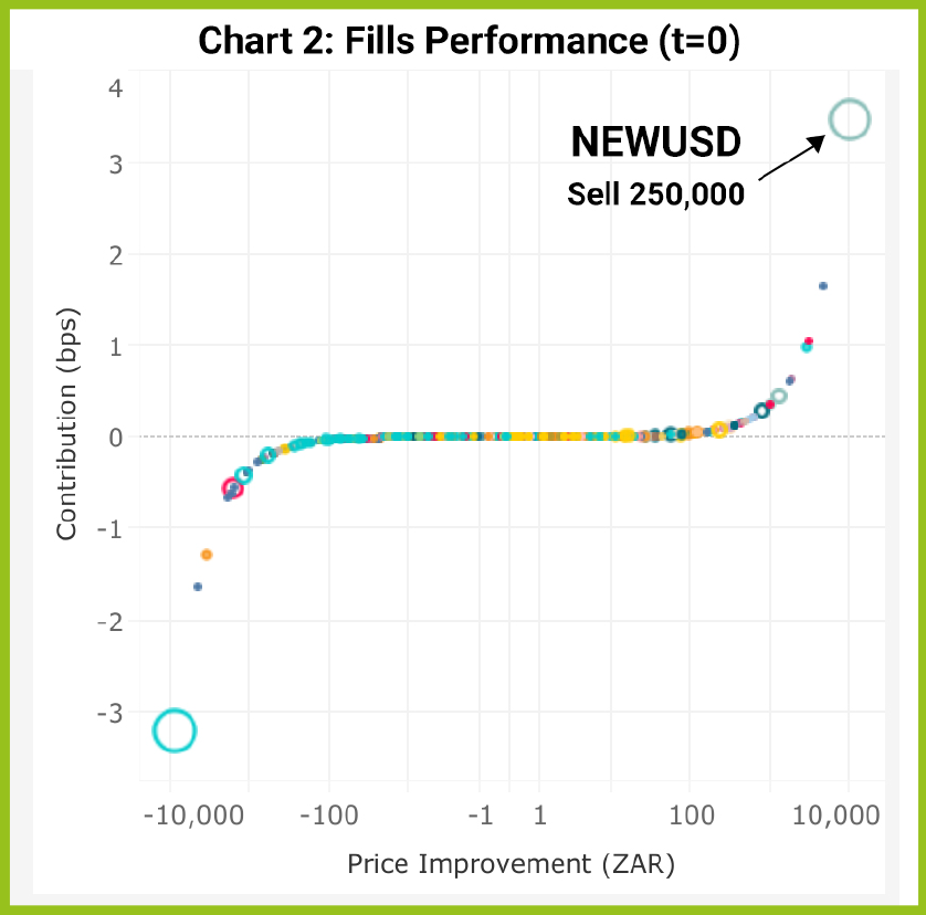
The chart also shows the contribution of each trade to the overall profitability of our Firm’s trading. This is measured on the y-axis. To calculate the contribution, we need to create a theoretical basket consisting of all the trades in our dataset with an adjusted execution price equal to the mid at the time of execution. We use this theoretical basket as a benchmark, which would have a price improvement (or trading cost) of zero.
Measuring the Temporary Impact of our Own Trades
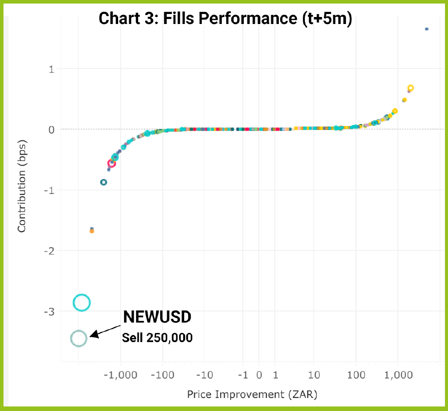
While the mid price at the time of execution gives us a reasonable benchmark for assessing our immediate trading cost or profit, it does not measure the longer term impact of our overall trading activity or that of other participants in the market. For this we can adjust the benchmark mid price by adjusting the filters and applying a series of time offsets (called ‘mark outs’) to measure the PnL of our trades against further changes to the share price.
Chart 3 shows Price Improvement using a 5 minute mark out for the same dataset. Our example trade in NEWUSD changes from being the best initial performer at t=0 to the worst performer with a loss of 10,000 ZAR and -3.45 bps contribution. The order in NEWUSD was a passive SELL order, meaning that the trade resulted from an aggressive buyer lifting the offer, and signalling their intention to the market. We can conclude that the price trend was upward, and the NEWUSD SELL trade turned to a negative performance (a process known as adverse selection).
Continuing the example, if the buyer had continued to send orders aggressively to the order book, the NEWUSD trade would have suffered ever greater costs. Although the buyer would be paying progressively higher prices the aggressive nature of the strategy would show as positive price improvement for the buyer, even though they are impacting the market price.
However, once the buyer has completed the trade, it is likely that the mid price will revert to or near to its original levels unless the market as a whole has decided on a new, higher fair value for the shares. If the market price reverts, we will see that the negative price improvement suffered by our seller of NEWUSD will reduce or become positive whilst the buyer will see their positive price improvement reduce or turn negative.
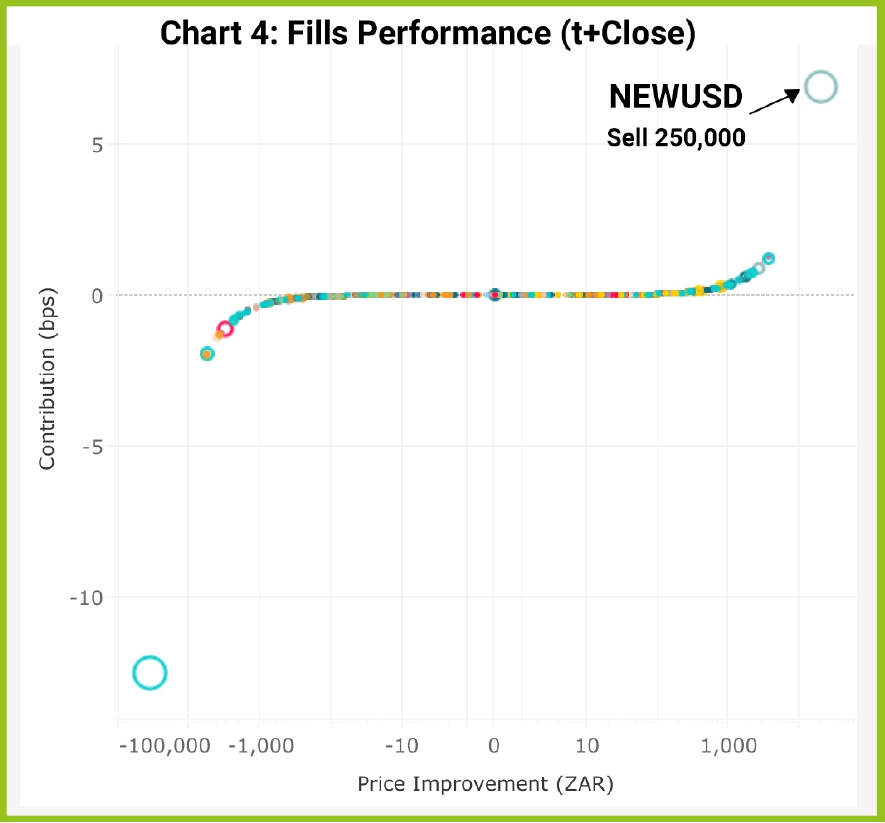
Spread Cost Analysis helps us to find out who has won the tug of war between the buyer and the seller by comparing the data using the mid at the time of the trade with the day’s closing price. In the final version of the scatter plot below, we see that our trade in NEWUSD has performed very well versus the Close price, more than overcoming the immediate 5 minute mark out cost, and returning 6.92 bps or 20,000 ZAR to the overall portfolio. If we were to review the buyer’s performance, we would see the opposite with a loss created by the trading strategy’s market impact.
Buys v Sells, Aggressive v Passive
By looking at overall trading performance, Spread Cost Analysis is able to help measure a Firm’s ability to correctly identify short term price movements and to efficiently place orders in the book by striking the balance between passive and aggressive orders. This analysis is most effective when used in conjunction with the other important related metrics provided by JSE Trade Explorer, such as average time to execute, order to fill ratio and order sizes. By making comparisons to Peer Group and Market Averages, the user can gain even better insights.
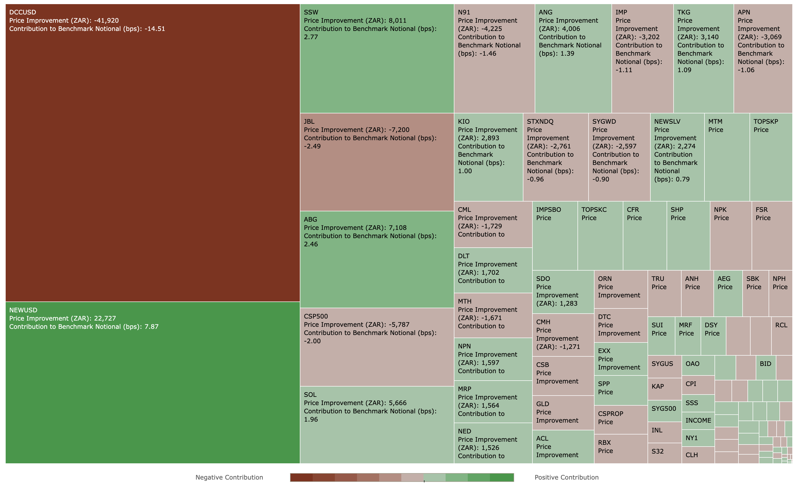
Spread Costs Analysis Heatmap
The heatmap helps to monitor and review trading performance with very large datasets by visualising the best and worst performing trades. The heatmap colour scheme shows which trades are the best and worst performers by absolute PnL while the block size the symbols which contribute the largest positive or negative PnL to the overall aggregated set of trades. This is also available as a per Sector view.
Summary
- JSE Trade Explorer provides the ability to analyse every trade by calculating the PnL of the execution price to the mid-point of the market at the time of a trade and a series of mark outs.
- For each trade, the contribution of this PnL to the aggregate set of trades for a Firm is also calculated, at the overall, sector and symbol level.
- By using mark out offsets, it is possible to isolate short term and long term trading cost and market impact of a trading strategy.
- Spread Cost Analysis should be used in Conjunction with other metrics and in particular the Order Analysis tools.
- Spread Cost Analysis should be used in Conjunction with other metrics and in particular the Order Analysis tools.
How To Access the Service
If you are an existing user of the JSE Trade Explorer, please follow this link and login using your existing credentials:
https://jse.big-xyt.com/loginIf you are a new user, please register for the service by following this link https://jse.big-xyt.com/signup and follow the instructions.
Feedback, Suggestions and Support
Please send feedback, questions or issues to [email protected] or use the form on the “Contact Us” link in the footer of all user views. We would appreciate as much information as possible such as:
- name of the window,
- any non-default filter settings,
- date range,
- symbol or stock selected.